You don’t need every data point to do PCA. I promise, it can work just as well even if you don’t interpolate first.
When you write a PhD dissertation, you end up spending a lot of time thinking about one very specific and esoteric topic. Every day. For years. Sometimes, you have to talk to someone outside of your research group, and when they ask what your dissertation is on, you confidently respond with the name of the problem you study, only to be met with a confused look and a misplaced sense of shock that they have no idea what you are talking about.
I get this cognitive dissonance everytime I tell someone my dissertation was on “matrix completion” and whenever someone mentions wanting to use PCA but having to deal with missing data points first. “You can do PCA without all the data”, I would exclaim, “it works better without interpolating!” Of course, the follow-up question to this point was always “how?”, and I had no good answer. Telling someone who is trying to solve a real problem that a technique works on paper is usually of no help.
Enter this blog post and the python package I made, SpaLoR. Amongst other features, SpaLor can do PCA when you have missing data by using matrix completion. In this tutorial, we’re going to use the Wisconsin breast cancer diagnostics dataset, which is included as an example dataset in scikit-learn. It consists of 30 morphological features from 569 breast tumour biopsies, along with a label of “malignant” or “benign”.
We start by loading in the data and necessary packages.
import numpy as np
import seaborn as sns

from sklearn.preprocessing import StandardScaler
from sklearn.decomposition import PCA
from sklearn.datasets import load_breast_cancer

breast_cancer = load_breast_cancer()
normalized_data = StandardScaler().fit_transform(breast_cancer.data)
There’s a reason this is a classic machine learning demonstration dataset: the features can predict the target variable using a linear model with incredibly high accuracy. When we do PCA and color the samples by diagnosis, we see an almost perfect seperation with just two principal components.
pca = PCA(n_components=2)
pca_data = pca.fit_transform(normalized_data)
ax=sns.scatterplot(x=pca_data[:,0], y=pca_data[:,1], hue=breast_cancer.target,s=10)
ax.set_xlabel("PC1")
ax.set_ylabel("PC2")
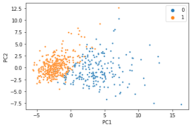
We were able to condense all 30 features into just two PCs, and the information we care about is still there. That’s less than 7% of the size of the original data, so it’s not too hard to believe that we don’t need 100% of the data to get a meaningful low-dimensional representation. Let’s simulate what would happen if 20% of the data was missing, and replaced with NaN.
What is Matrix Completion?
Simply put, the goal of matrix completion is fill in missing entries of a matrix (or dataset) given the fact that the matrix is low rank, or low dimensional. Essentially, it’s like a game of Sudoku with a different set of rules. Lets say I have a matrix that I know is supposed to be rank 2. That means that every column can be written as a linear combination (weighted sum) of two vectors. Lets look at an example of what this puzzle might look like.
\[\begin{bmatrix} 1 & 1 &2 & 2\\2&1&3&-\\1&2&-&1 \end{bmatrix}\]
The first two columns are completly filled in, so we can use those to figure out the rest of the columns. Based on the few entries in the third column that are given, we can see that the third column should probably be the first column plus the second column. Likewise, the fourth column is two times the first column minus the second column.
\[\begin{bmatrix} 1 & 1 &2 & 2\\2&1&3&5\\1&2&3&1 \end{bmatrix}\]
That was a particularly easy example since we knew the first two columns completely.
To see why we should care about this, here’s a claim that shouldn’t be too hard to believe: Datasets are inherently low rank . In the example we just did, the columns could be movies, the rows could be people, and the numbers could be how each person rated each movie. Obviously, this is going to be sparse since not everyone has seen every movie. That’s where matrix completions comes in. When we filled in the missing entries, we gave our guess as to what movies people are going to enjoy. After explaining an algorithm to do matrix completion, we’re going to try this for a data set with a million ratings people gave movies and see how well we recommend movies to people.
How do we do it?
There’s two paradigms for matrix completion. One is to minimize the rank of a matrix that fits our measurements, and the other is to find a matrix of a given rank that matches up with our known entries. In this blog post, I’ll just be talking about the second.
Before we explain the algorithm, we need to introduce a little more notation. We are going to let \(\Omega\) be the set of indices where we know the entry. For example, if we have the partially observed matrix
\[\begin{matrix}\color{blue}1\\\color{blue}2\\\color{blue}3\end{matrix}\begin{bmatrix} & 1 & \\ & & 1\\1 & & \end{bmatrix}\]
\[\begin{matrix} &\color{red}1 & \color{red}2 & \color{red}3 \end{matrix}\]
then, \(\Omega\) would be \(\{ (\color{blue} 1, \color{red}2), (\color{blue}2 , \color{red}3),(\color{blue} 3, \color{red}1)\}\) We can now pose the problem of finding a matrix with rank \(r\) that best fits the entries we’ve observe as an optimization problem.
\[\begin{aligned}&\underset{X}{\text{minimize}}& \sum_{(i,j)\text{ in }\Omega} (X_{ij}-M_{ij})^2 \\& \text{such that} & \text{rank}(X)=r\end{aligned}\]
The first line specifies objective function (the function we want to minimize), which is the sum of the square of the difference between \(X_{ij}\) and \(M_{ij}\) for every \((i,j)\) that we have a measurement for. The second line is our constraint, which says that the matrix has to be rank \(r\) .
While minimizing a function like that isn’t too hard, forcing the matrix to be rank \(r\) can be tricky. One property of a low rank matrix that has \(m\) rows and \(n\) columns is that we can factor it into two smaller matrices like such:
\[X=UV\]
where \(U\) is \(n\) by \(r\) and \(V\) is \(r\) by \(m\) . So now, if we can find matrices \(U\) and \(V\) such that the matrix \(UV\) fits our data, we know its going to be rank \(r\) and that will be the solution to our problem.
If \(u_i\) is the \(i^{th}\) column of \(U\) and \(v_j\) is the \(j^{th}\) column of \(V\) , then \(X_{ij}\) is the inner product of \(u_i\) and \(v_j\) , \(X_{ij}= \langle u_i, v_i \rangle\) . We can rewrite the optimization problem we want to solve as
\[\begin{aligned} \underset{U, V}{\text{minimize}}& \sum_{(i,j)\in \Omega} (\langle u_i, v_i \rangle-M_{ij})^2 \end{aligned}\]
In order to solve this, we can alternate between optimizing for \(U\) while letting \(V\) be a constant, and optimizing over \(V\) while letting \(U\) be a constant. If \(t\) is the iteration number, then the algorithm is simply
\[\begin{aligned} \text{for } t=1,2,\ldots:& \\ U^{t}=&\underset{U}{\text{minimize}}& \sum_{(i,j)\in \Omega} (\langle u_i, v^{t-1} i \rangle-M_{ij})^2 \\ V^{t}=&\underset{ V}{\text{minimize}}& \sum_{(i,j)\in \Omega} (\langle u^t_i, v_i \rangle-M_{ij})^2 \\ \end{aligned}\]
At each iteration, we just need to solve a least squares problem which is easy enough.